pyIBLM

Interpretable Boosted Linear Models

Author

Paul Beard and Karol Gawlowski

Published

May 23, 2026

Installation

pyIBLM can be installed from PyPI:

pip install pyiblm

To use load_freMTPL2freq() you will also need the optional data dependency:

pip install "pyiblm[data]"

Introduction

pyIBLM stands for “Interpretable Boosted Linear Model”.

An IBLM is essentially a hybrid model consisting of two components:

Generalised Linear Model (GLM) — fitted to the training data
Booster Model¹ — fitted to the residuals of the training data against GLM predictions in step 1.

The purpose of this article is to show you how to use pyIBLM to train, explain, and predict.

Theory

The overall process for fitting and interpreting an IBLM is as follows:

Step 1: Fit a GLM

\[ g(\mu) = \beta_0 + \beta_1 x_1 + \beta_2 x_2 + \cdots + \beta_n x_n \]

Where \(g(\cdot)\) is the link function, \(\mu\) is the expected value of the response, and \(\beta\) values are your standard regression coefficients.

\[ \text{GLM prediction} = g^{-1} (\beta_0 + \beta_1 x_1 + \beta_2 x_2 + \cdots + \beta_n x_n) \]

Step 2: Train a Booster on GLM’s Errors

Train a booster model (XGBoost) on the residuals of the actual response values against the GLM predictions.

Step 3: Use SHAP to Break Down the Booster

SHAP decomposition allows the booster’s prediction to be apportioned into contributions from each feature:

\[ \text{Booster prediction} = g^{-1} (\varphi_0 + \varphi_1(x) + \varphi_2(x) + \cdots + \varphi_n(x)) \]

Where \(\varphi_j(x)\) is how much feature \(j\) contributed to a specific prediction.

Step 4: Convert SHAP Values to Beta Coefficient Corrections

Transform each SHAP contribution into beta corrections:

\[ \alpha_j(x) \approx \frac{\varphi_j(x)}{x_j} \]

There are two situations where \(\alpha_j(x)\) is set to zero and \(\varphi_j(x)\) is added to the intercept instead — when \(x\) is a numerical variable and its value is zero, or when \(x\) is a categorical variable and its value is the reference level².

\[ \begin{aligned} \alpha_j(x) &= 0 \text{ when } \begin{cases} x_j = 0 & \text{(numerical)} \\ x_j = \text{ref} & \text{(categorical)} \end{cases} \\[1em] \alpha_0(x) &= \sum_{\substack{j: x_j = 0 \\ \text{or } x_j = \text{ref}}} \varphi_j(x) \end{aligned} \]

Step 5: Combine

The final IBLM can be interpreted as a collection of adjusted GLMs. Each row of the data will essentially have its own GLM coefficients — the sum of:

The GLM coefficients derived in step 1, which are the same for all rows
The beta corrections derived in step 4, which are unique to that predictor variable combination.

\[ g(\mu) = (\beta_0 + \varphi_0 + \alpha_0) + (\beta_1 + \alpha_1(x))x_1 + (\beta_2 + \alpha_2(x))x_2 + \cdots + (\beta_n + \alpha_n(x))x_n \]

\[ \begin{aligned} g(\mu) &= \beta'_0 + \beta'_1 x_1 + \beta'_2 x_2 + \cdots + \beta'_n x_n \\ \text{where } \beta'_j &= \beta_j + \alpha_j(x) \\ \text{and } \beta'_0 &= \beta_0 + \varphi_0 + \alpha_0 \end{aligned} \]

The IBLM prediction combines components:

\[ \begin{aligned} \text{IBLM prediction} &= g^{-1} (\beta'_0 + \beta'_1 x_1 + \beta'_2 x_2 + \cdots + \beta'_n x_n) \\[0.5em] &= \begin{cases} \text{GLM prediction} \times \text{Booster prediction} & \text{when } g = \log \\ \text{GLM prediction} + \text{Booster prediction} & \text{when } g = \text{identity} \end{cases} \end{aligned} \]

This preserves the familiar GLM form while incorporating the booster’s superior predictive power.

Train

To train an IBLM we must get our data into an appropriate format. In this document our demonstrations will be completed using the French motor claims dataset freMTPL2freq. For simplicity, we will drop the "Exposure" column and assume all rows carry equal weight. In practice however this should be allowed for either through weight_var or offset_var (see Offsetting and Weighting).

Data for training an IBLM must be in the form of a dict of three DataFrames with keys "train", "validate" and "test". The function split_into_train_validate_test() can conveniently split a single DataFrame into such a structure.

Code

freMTPL2freq = load_freMTPL2freq()

df_dict = split_into_train_validate_test(
    freMTPL2freq.drop(columns=["Exposure"]),
    seed=1,
)

The IBLM class has currently one method available to train it: IBLM.fit(). This method uses XGBoost as the booster model, performing steps 1 and 2 of the Theory.

The output is an object of class IBLM. It contains two component models: glm_model and booster_model, along with other metadata (see the IBLM.fit() docstring for full details).

Code

iblm_model = IBLM()

iblm_model = iblm_model.fit(
    df_dict,
    response_var="ClaimNb",
    family="poisson",
    params={"seed": 1},
)

type(iblm_model)

iblm._model.IBLM

For convenience, it is also possible to train an XGBoost model using the same settings as your IBLM. This can be useful when directly comparing models (for example see Pinball Score).

Code

xgb_model = train_xgb_as_per_iblm(iblm_model)

Explain

Code to explain and interpret an IBLM object is provided through the ExplainIBLM class. This performs steps 3, 4 and 5 of the Theory. The values derived are all based on the data fed in, which would usually be the test portion of your dataset.

Code

explainer = ExplainIBLM(iblm_model, df_dict["test"])

The ExplainIBLM object exposes the following attributes:

shap — DataFrame of raw SHAP values (\(\varphi_n(x)\) from step 3 of Theory)
beta_corrections — DataFrame of beta corrections in wide/one-hot format (\(\alpha_0(x)\) and \(\alpha_j(x)\) from step 4)
data_beta_coeff — DataFrame of corrected beta coefficients (\(\beta'_0\) and \(\beta'_j\) from step 5). For categorical variables, the value corresponds to the relevant coefficient for that datapoint.

And the following plotting methods:

beta_corrected_scatter() — scatter or boxplot of corrected beta coefficients vs variable values
beta_corrected_density() — density plot of corrected beta coefficients
bias_density() — density plot of SHAP values migrated to the bias
overall_correction() — distribution of the booster’s overall correction

Beta Corrected Density

The corrected beta coefficients (\(\beta'_j\)) can be observed in a density plot. This allows you to see corrected beta coefficient values for a particular variable.

The density plot also shows the standard error for the original beta coefficient fitted in the GLM component, which helps in understanding the significance of the range in corrected beta coefficients.

Numerical Variables

For numerical variables, calling the method returns a single figure. Below we show examples for different numerical variables in freMTPL2freq.

Code

explainer.beta_corrected_density("VehPower");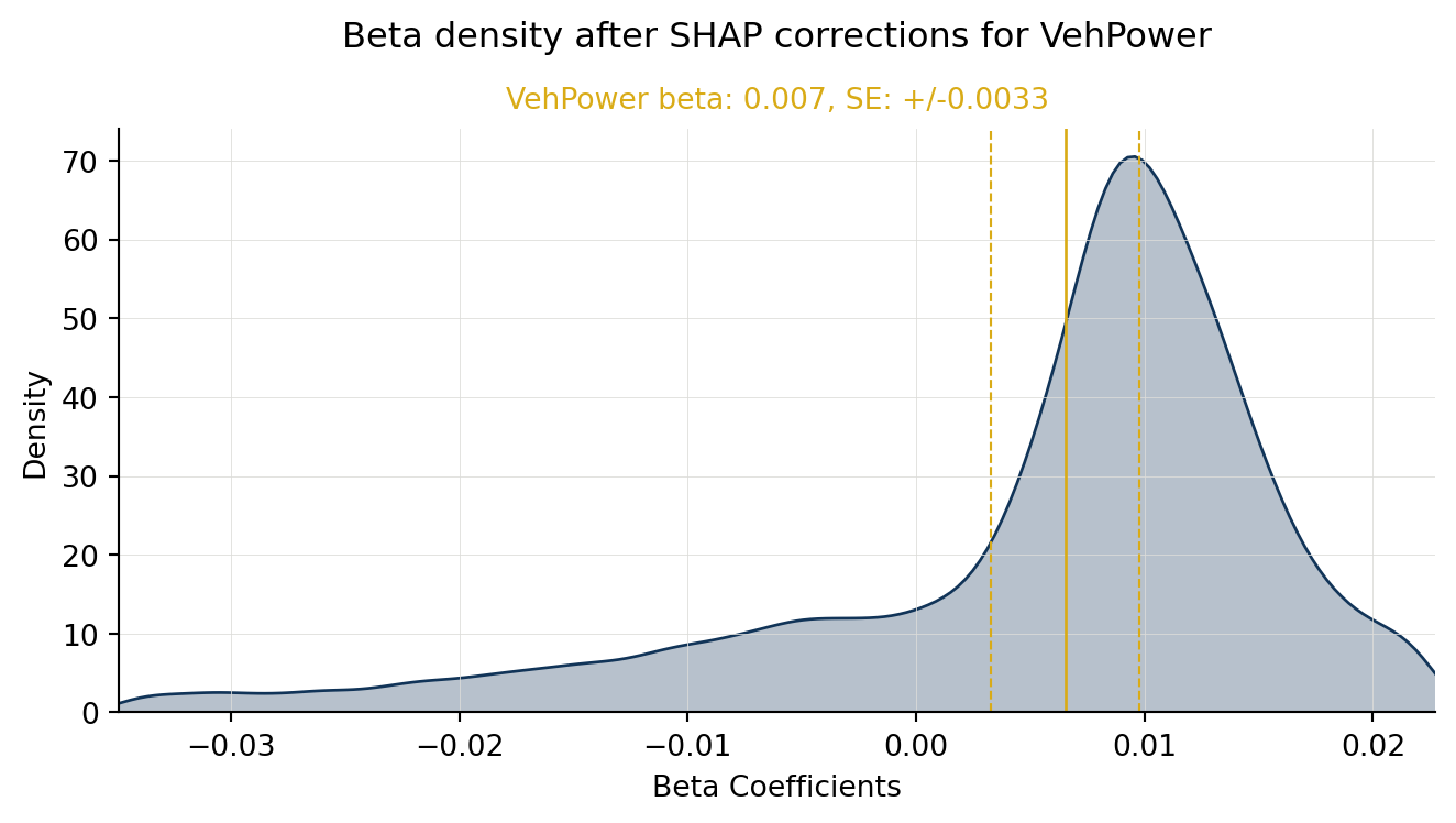

Code

explainer.beta_corrected_density("VehAge");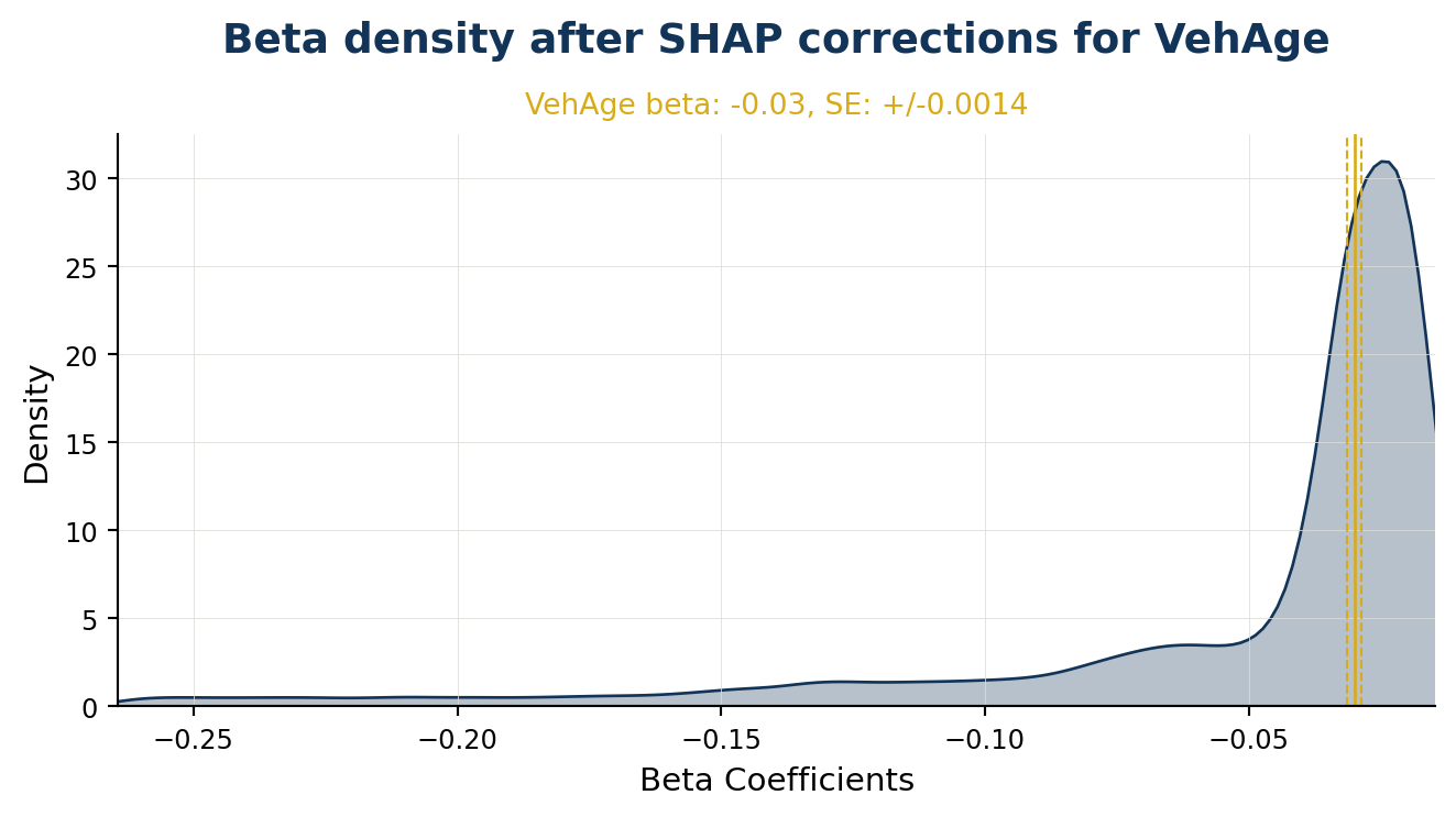

Code

explainer.beta_corrected_density("DrivAge");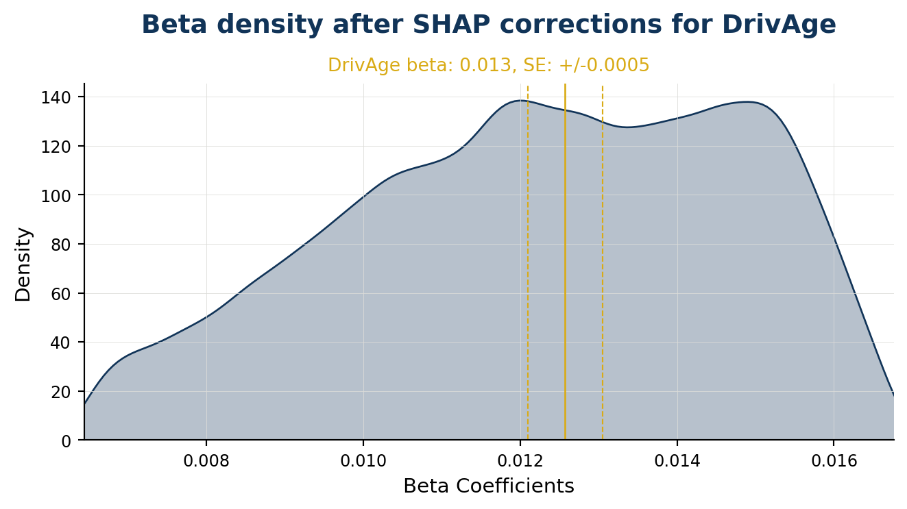

Code

explainer.beta_corrected_density("BonusMalus");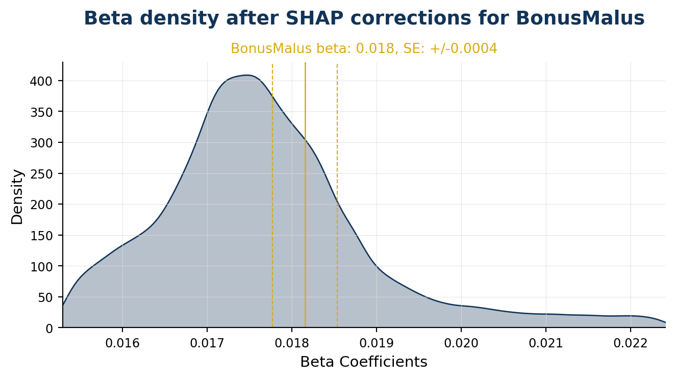

Categorical Variables

For categorical variables, calling the method returns a dict of figures — one per level, excluding the reference level.

In the example below "VehBrand" has 11 levels and produces 10 figures. Level "B1" is the reference level and does not have a beta coefficient in the GLM component; instead, its SHAP values are migrated to the bias (see Bias Corrected Density).

Code

import base64, io
from IPython.display import HTML

veh_brand_plots = explainer.beta_corrected_density("VehBrand", type="hist")

figs = list(veh_brand_plots.values())
for i in range(0, len(figs), 2):
    pair = figs[i:i+2]
    imgs = ""
    for f in pair:
        buf = io.BytesIO()
        f.savefig(buf, format="png", bbox_inches="tight")
        encoded = base64.b64encode(buf.getvalue()).decode()
        imgs += f'<img src="data:image/png;base64,{encoded}" style="width:{100 // len(pair)}%">'
        plt.close(f)
    display(HTML(f'<div style="display:flex;gap:4px">{imgs}</div>'))

Beta Corrected Scatter

The corrected beta coefficients (\(\beta'_j\)) can be observed in a scatter plot (or boxplot). This allows you to see corrected beta coefficient values for a particular variable and their relationship to that variable’s value.

Numerical Variables

When varname is set to a numerical variable, a scatter plot is produced. The example below shows corrected beta coefficient values against driver age. The original beta coefficient from the GLM component is shown as a dashed black line (and stated near the top of the plot in orange). A smoothed trend line shows the overall pattern of correction.

The color argument can be set to observe interactions with a second variable.

Code

explainer.beta_corrected_scatter("DrivAge", color="VehPower");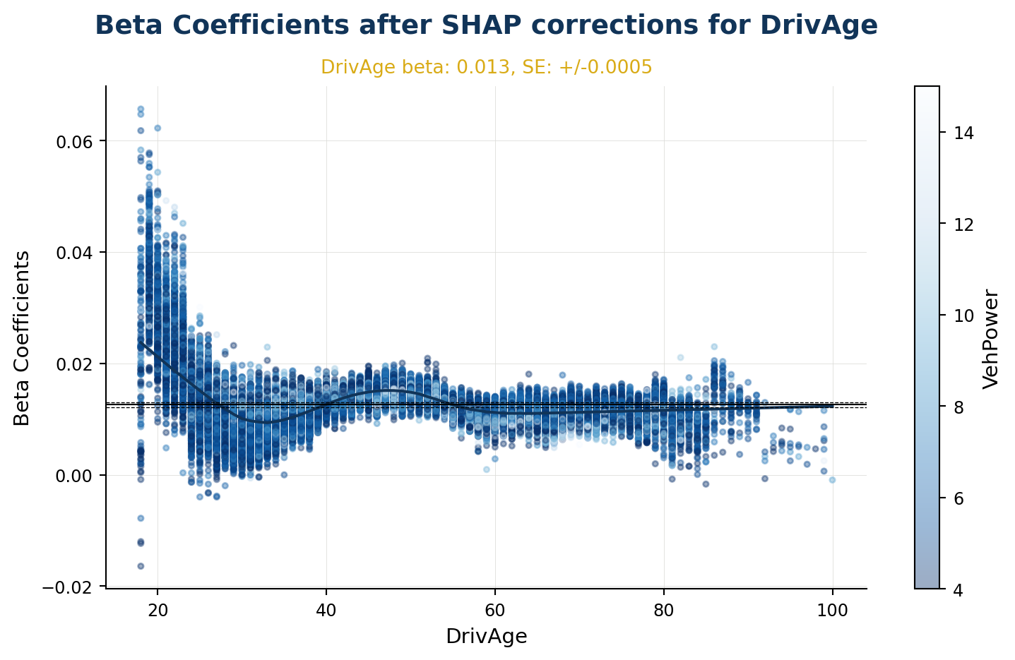

Categorical Variables

When varname is set to a categorical variable, a boxplot is produced showing the distribution for each level.

Code

explainer.beta_corrected_scatter("VehBrand");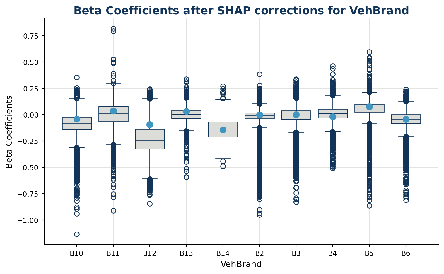

Bias Corrected Density

As described in step 4 of Theory, some SHAP values cannot be translated to beta corrections and are instead migrated to the bias. There are two situations where this occurs:

A numerical variable where the value was zero for that data point.
A categorical variable where the value was the reference level for that data point.

The bias_density() method returns a dict with two figures:

"bias_correction_var" — shows all individual instances of bias migration across variables in the test dataset. For categorical variables, counts in each facet equal the occurrences of the reference level. For numerical variables, counts equal the occurrences of zero.
"bias_correction_total" — the cumulative sum of these components across each data point. The standard bias value and its standard error are shown as a solid blue line with dashed orange bounds.

Code

bias_corrections = explainer.bias_density()
plt.close("all")
display(bias_corrections["bias_correction_var"])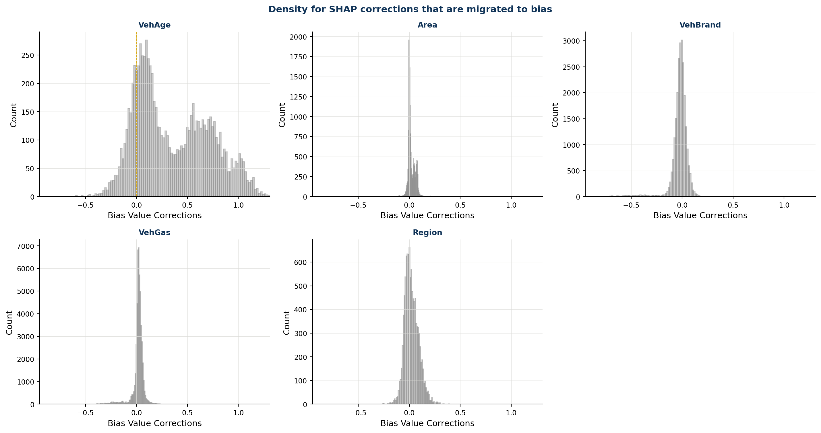

Code

display(bias_corrections["bias_correction_total"])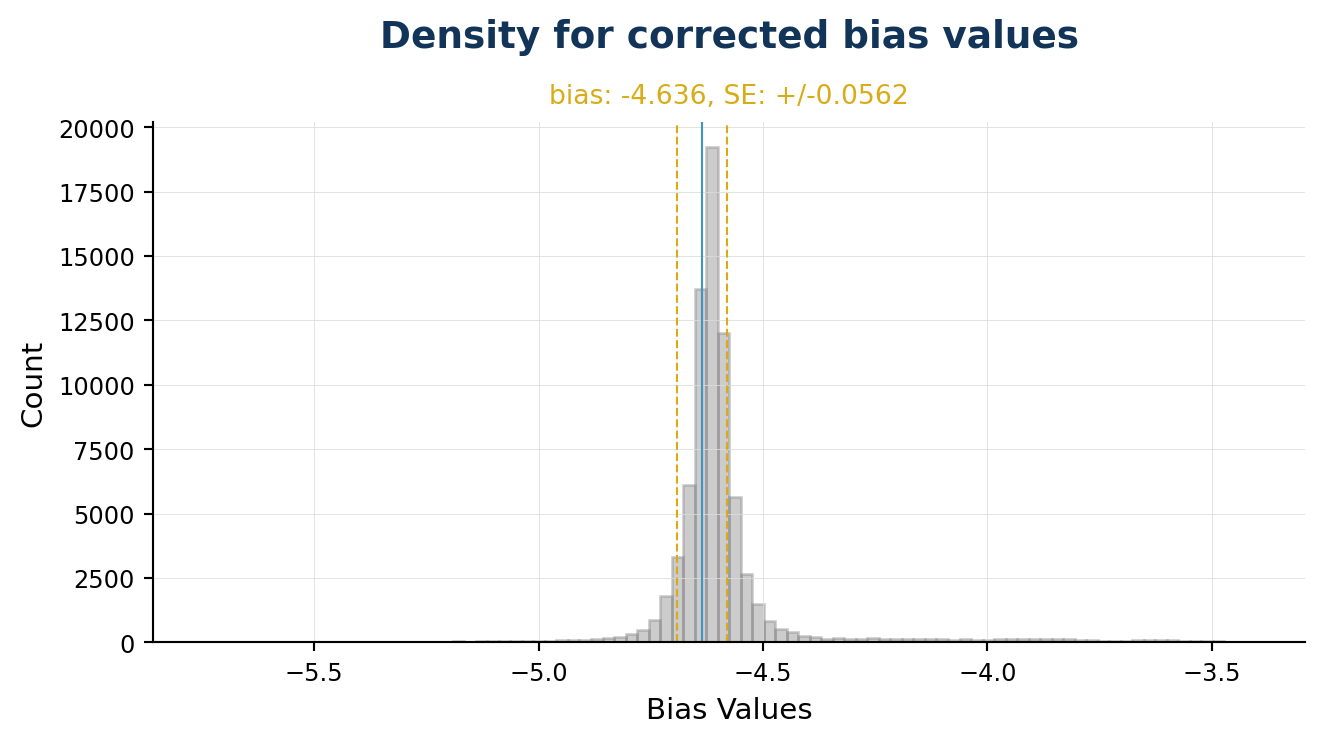

Overall Correction

The distribution of overall corrections across your test data can be observed. If the link function is log, the correction is a multiplier (as below). If the link function is identity, the correction is an addition. By default the x axis is transformed by the link function.

Code

explainer.overall_correction();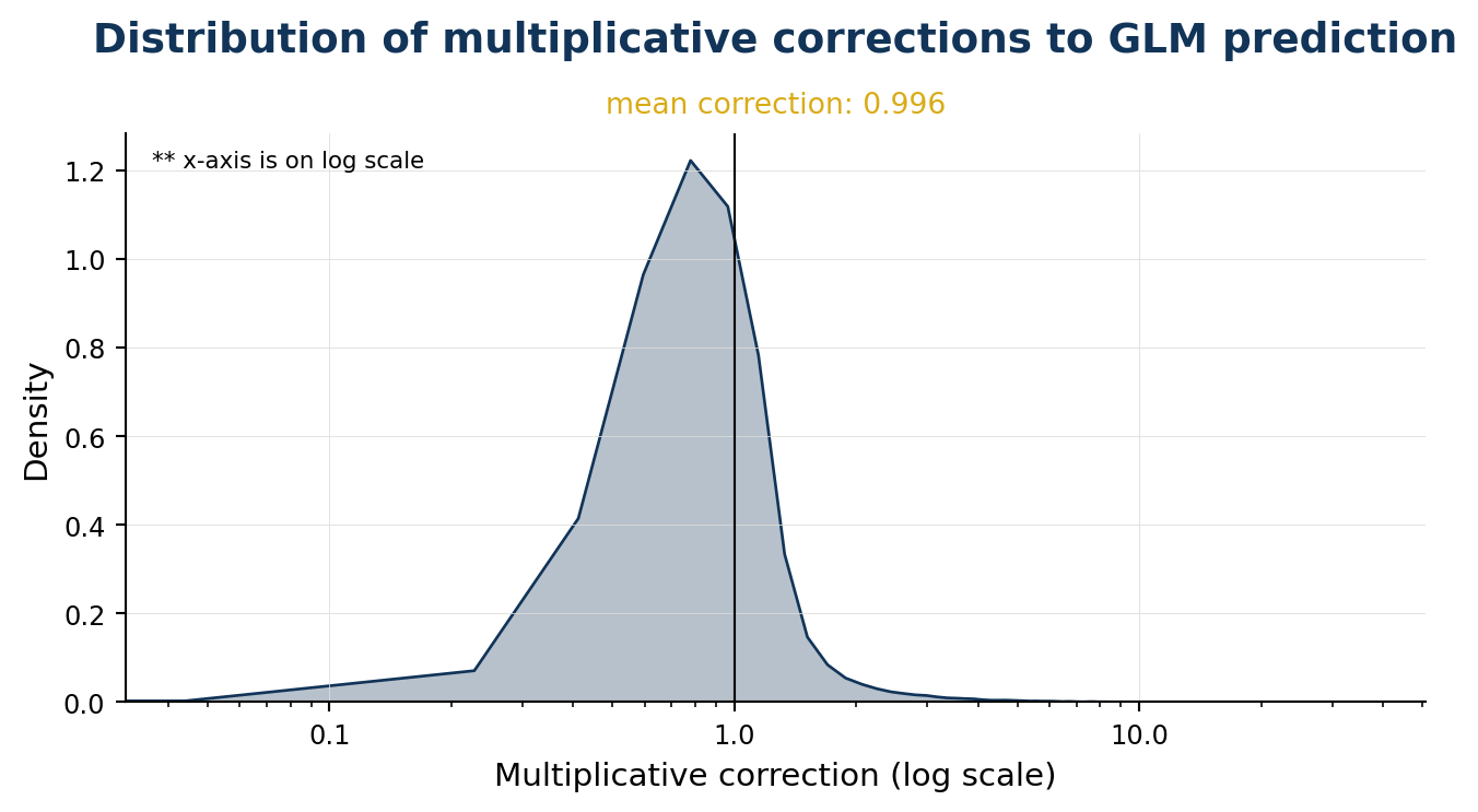

Code

explainer.overall_correction(transform_x_scale_by_link=False);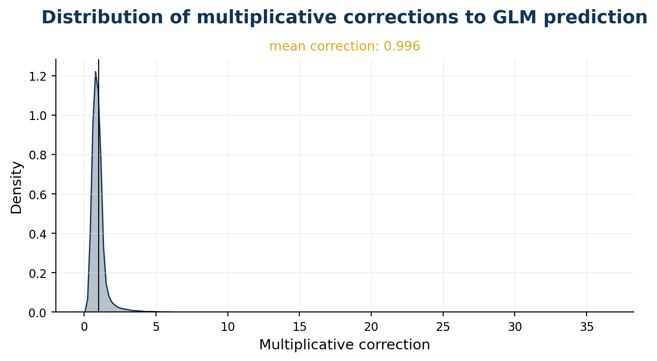

Predict

The IBLM class provides a predict() method that applies both the glm_model and booster_model components.

Code

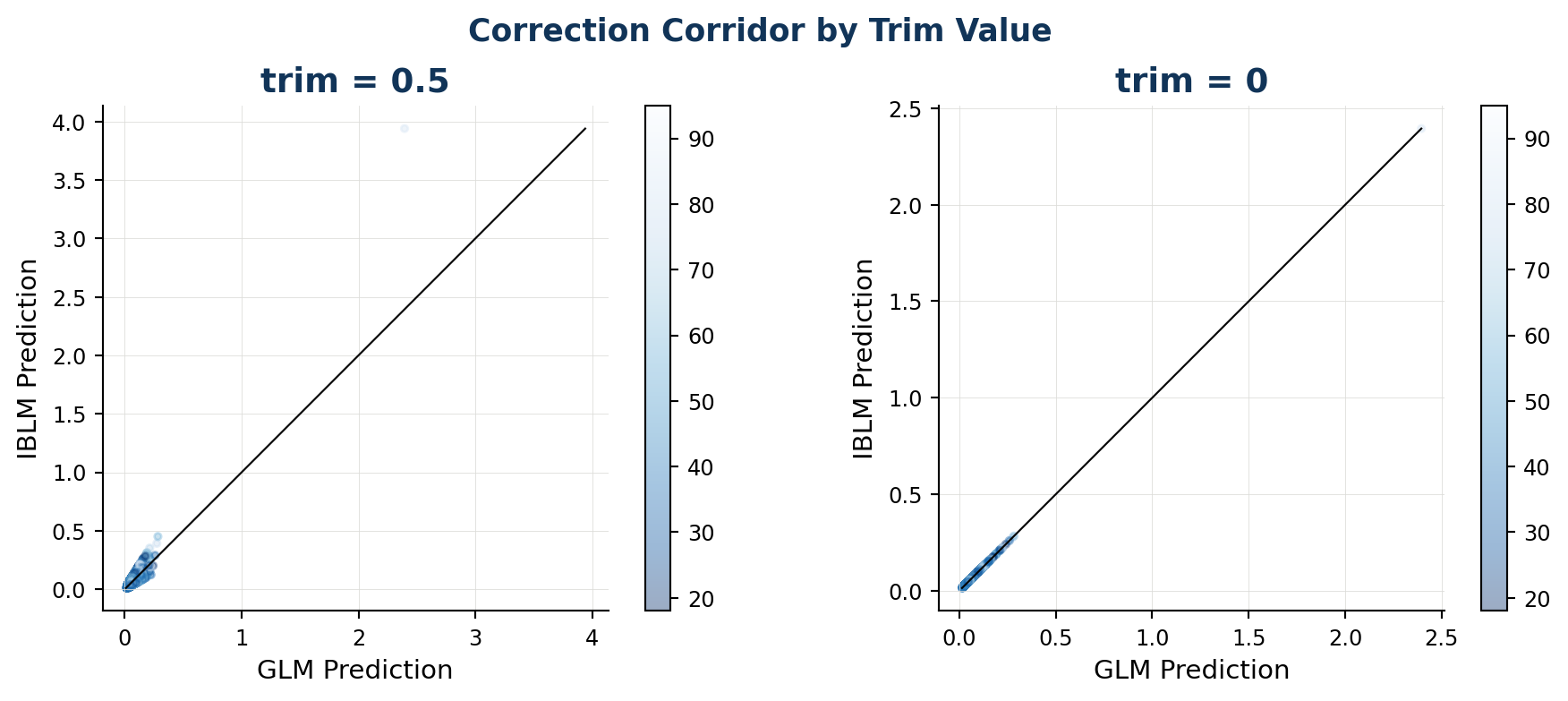
predictions = iblm_model.predict(df_dict["test"])

The predict method contains a trim option which truncates the booster model predictions to prevent extreme deviation from the foundation GLM. This is explored further in Correction Corridor.

Because an IBLM is essentially a collection of GLMs, and the corrected beta coefficients are derived by ExplainIBLM, it is also possible to predict through linear calculation:

Code

cols_to_drop = [iblm_model.response_var]

coeff_multiplier = df_dict["test"].drop(columns=cols_to_drop).copy()
for col in iblm_model.predictor_vars["categorical"]:
    coeff_multiplier[col] = 1
coeff_multiplier.insert(0, "bias", 1)

predictions_alt = (
    (explainer.data_beta_coeff * coeff_multiplier)
    .sum(axis=1)
    .pipe(np.exp)
    .values
)

# difference in predictions very small between two alternative methods
pd.Series(predictions_alt / np.array(predictions, dtype=float) - 1).describe()

count    101934.0
mean          0.0
std           0.0
min     -0.000001
25%          -0.0
50%           0.0
75%           0.0
max      0.000002
dtype: Float64

Pinball Score

The pinball score measures model performance as the improvement in predictability compared to using the training data mean. A higher score is better. In the example below the IBLM has an improved score compared to the GLM. We also add the xgb_model (derived in Train) as a further comparison.

Code

get_pinball_scores(
    data=df_dict["test"],
    iblm_model=iblm_model,
    additional_models={"xgb": xgb_model},
)

	model	poisson_deviance	pinball_score
0	homog	0.321667	0.000000
1	glm	0.315859	0.018055
2	iblm	0.301503	0.062687
3	xgb	0.301210	0.063596

Correction Corridor

The correction_corridor() function applies predict() with different trim settings and plots the results. When trim is zero, the IBLM predictions are the same as the GLM predictions. The color argument can be set to observe any patterns.

Code

correction_corridor(
    iblm_model,
    df_dict["test"],
    trim_vals=[0.5, 0],
    sample_perc=0.1,
    color="DrivAge",
);

Offsetting and Weighting

In the examples above using freMTPL2freq, we dropped the "Exposure" column and treated each row equally. In reality we would want to account for the fact that some periods carry more weight than others. We can do this either through offset_var or weight_var.

Offsetting

Offsetting in pyIBLM works similarly to offsetting in a GLM. Any offset specified is incorporated only into the glm_model and not the booster_model component.

For a Poisson distribution we can implement offsetting to place more value on rows with greater Exposure.

To do this, create a column in your data for the offset. For Poisson, quasipoisson, Gamma or Tweedie families this must be in log-transformed form. Take care to drop any unneeded columns (here "Exposure" once it has been used to create "LogExposure").

Code

df_dict_offset = split_into_train_validate_test(
    freMTPL2freq.assign(LogExposure=lambda df: np.log(df["Exposure"]))
                .drop(columns=["Exposure"]),
    seed=1,
)

iblm_model_offset = IBLM()

iblm_model_offset = iblm_model_offset.fit(
    df_dict_offset,
    response_var="ClaimNb",
    offset_var="LogExposure",
    family="poisson",
    params={"seed": 0},
)

By adding an offset_var the fitted object will have an offset_var attribute. The glm_model is fitted with this offset. The booster model is trained on the GLM residuals, so the offset is implicitly applied rather than explicitly included.

When using predict() or ExplainIBLM, the offset column is accounted for automatically. If it is not present in the test data, an offset of zero is assumed:

Code

# set offset to zero (recommended for Poisson rate predictions)
predict_offset_a = iblm_model_offset.predict(
    df_dict_offset["test"].assign(LogExposure=0)
)

# ...or simply drop the column — treated as zero
predict_offset_b = iblm_model_offset.predict(
    df_dict_offset["test"].drop(columns=["LogExposure"])
)

(predict_offset_a == predict_offset_b).all()  # True

np.True_

If you leave the offset_var in the data, predictions are based on it:

Code

# predictions based on LogExposure column
predict_offset_c = iblm_model_offset.predict(df_dict_offset["test"])

(predict_offset_a == predict_offset_c).all()  # False — uses LogExposure values

np.False_

Note the same applies to get_pinball_scores() and correction_corridor().

Weighting

An alternative is to use the weight feature. Note that for this to work the response variable must be the claim rate rather than the claim count.

Code

df_dict_weight = split_into_train_validate_test(
    freMTPL2freq.assign(ClaimRate=lambda df: df["ClaimNb"] / df["Exposure"])
                .drop(columns=["ClaimNb"]),
    seed=1,
)

iblm_model_weight = IBLM()

iblm_model_weight = iblm_model_weight.fit(
    df_dict_weight,
    response_var="ClaimRate",
    weight_var="Exposure",
    family="quasipoisson",
    params={"seed": 0},
)

By adding a weight_var the fitted object will have a weight_var attribute. Both the glm_model and booster_model are fitted with this weight applied. When using predict() or ExplainIBLM, the weight column is not used in the prediction:

Code

# weight_var is ignored in predict()
predict_weight_a = iblm_model_weight.predict(df_dict_weight["test"])

# ...or simply drop the column — makes no difference
predict_weight_b = iblm_model_weight.predict(
    df_dict_weight["test"].drop(columns=["Exposure"])
)

(predict_weight_a == predict_weight_b).all()  # True

np.True_

Note that for get_pinball_scores() the weight_var is considered when present. When absent, an equal weight of 1 is assumed for each row. It is recommended to include the weight variable if available.

Code

# with weight
ps_weight_a = get_pinball_scores(df_dict_weight["test"], iblm_model_weight)

# without weight (equal weighting assumed)
ps_weight_b = get_pinball_scores(
    df_dict_weight["test"].drop(columns=["Exposure"]),
    iblm_model_weight,
)

ps_weight_a.equals(ps_weight_b)  # False — ps_weight_a is weighted by Exposure

False

Footnotes

pyIBLM uses XGBoost as the booster model.↩︎
The reference level of a categorical variable is the value for which there is no coefficient in the GLM. Reference levels can be found in iblm_model.cat_levels["reference"].↩︎