Density Plot of Bias Corrections from SHAP values
Source:R/create_beta_correction_plot_functions.R
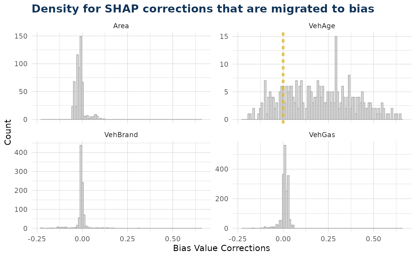
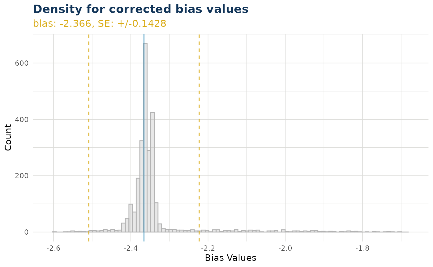
bias_density.RdVisualizes the distribution of SHAP corrections that are migrated to bias terms, showing both per-variable and total bias corrections.
NOTE This function signature documents the interface of functions created by create_bias_density.
Value
A list with two ggplot objects:
bias_correction_var: Faceted plot showing bias correction density from each variable. Note that variables with no records contributing to bias correction are dropped from the plot.bias_correction_total: Plot showing total corrected bias density.
Examples
# This function is created inside explain_iblm() and is output as an item
df_list <- freMTPLmini |>
dplyr::mutate(LogExposure = log(Exposure), .keep = "unused") |>
split_into_train_validate_test(seed = 9000)
iblm_model <- train_iblm_xgb(
df_list,
response_var = "ClaimNb",
offset_var = "LogExposure",
family = "poisson"
)
explain_objects <- explain_iblm(iblm_model, df_list$test)
explain_objects$bias_density()
#> $bias_correction_var
 #>
#> $bias_correction_total
#>
#> $bias_correction_total
 #>
# This function must be created, and cannot be called directly from the package
try(
bias_density()
)
#> Error in bias_density() :
#> This function documents the interface only and cannot be called
#> directly. Instead, try one of the following
#> ℹ Use explain_iblm()$bias_density()
#> ℹ Call a function output from create_bias_density()
#>
# This function must be created, and cannot be called directly from the package
try(
bias_density()
)
#> Error in bias_density() :
#> This function documents the interface only and cannot be called
#> directly. Instead, try one of the following
#> ℹ Use explain_iblm()$bias_density()
#> ℹ Call a function output from create_bias_density()