Creates a list that explains the beta values, and their corrections, of the ensemble IBLM model
Arguments
- iblm_model
An object of class 'iblm'. This should be output by `train_iblm_xgb()`
- data
Data frame.
If you have used `split_into_train_validate_test()` this will be the "test" portion of your data.
- migrate_reference_to_bias
Logical, migrate the beta corrections to the bias for reference levels? This applied to categorical vars only. It is recommended to leave this setting on TRUE
Value
A list containing:
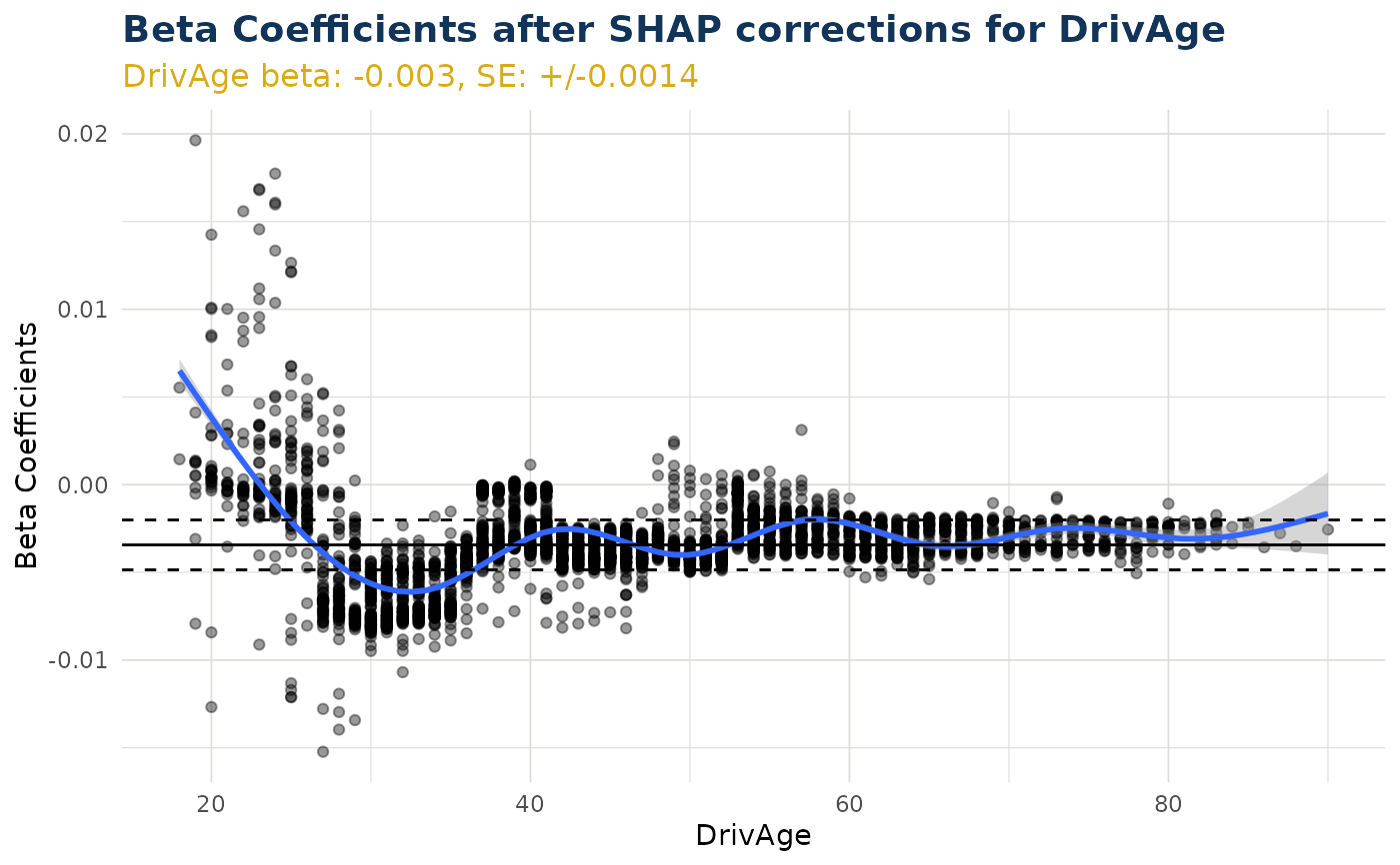
- beta_corrected_scatter
Function to create scatter plots showing SHAP corrections vs variable values (see
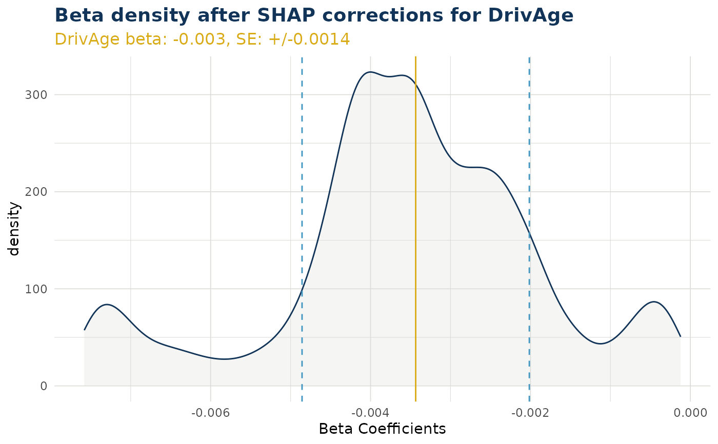
beta_corrected_scatter)- beta_corrected_density
Function to create density plots of SHAP corrections for variables (see
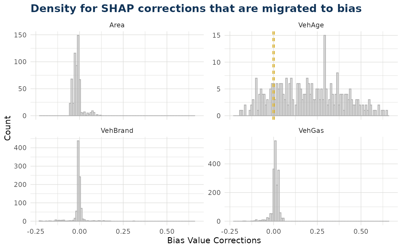
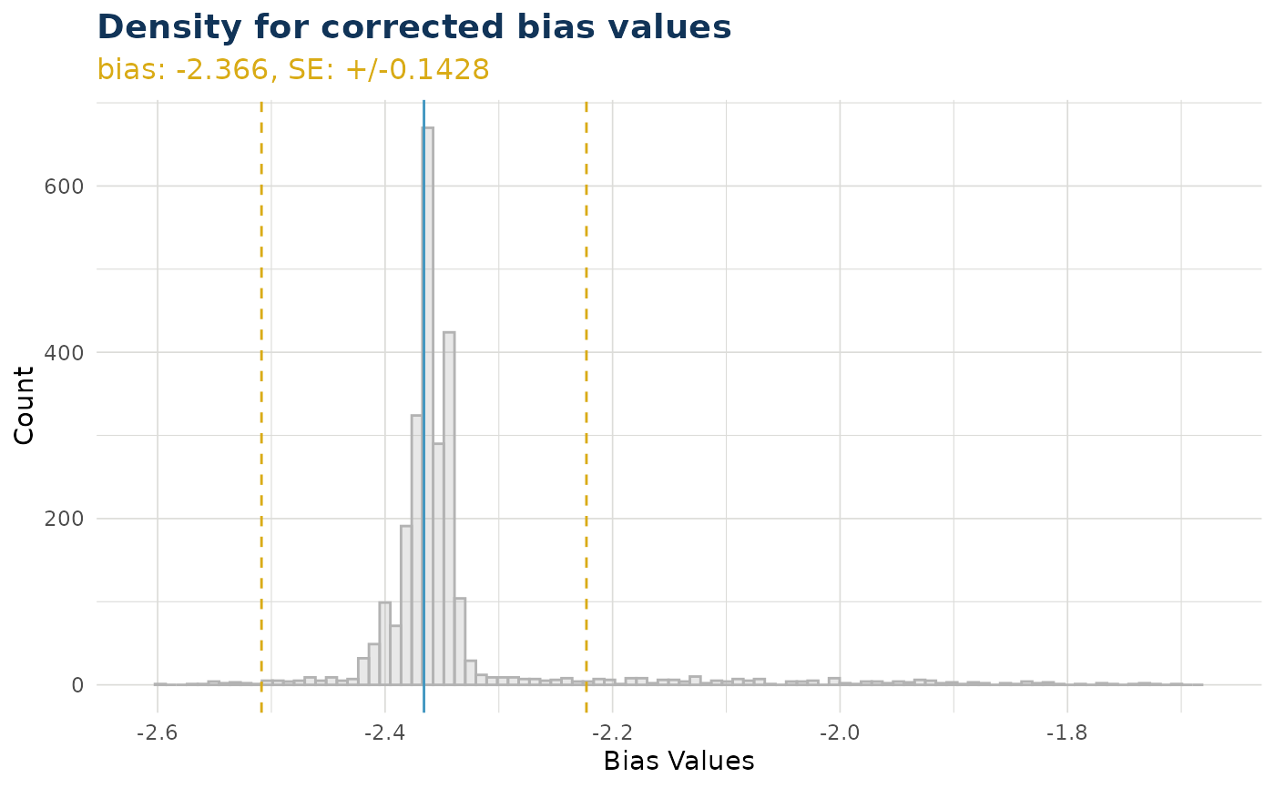
beta_corrected_density)- bias_density
Function to create density plots of SHAP corrections migrated to bias (see
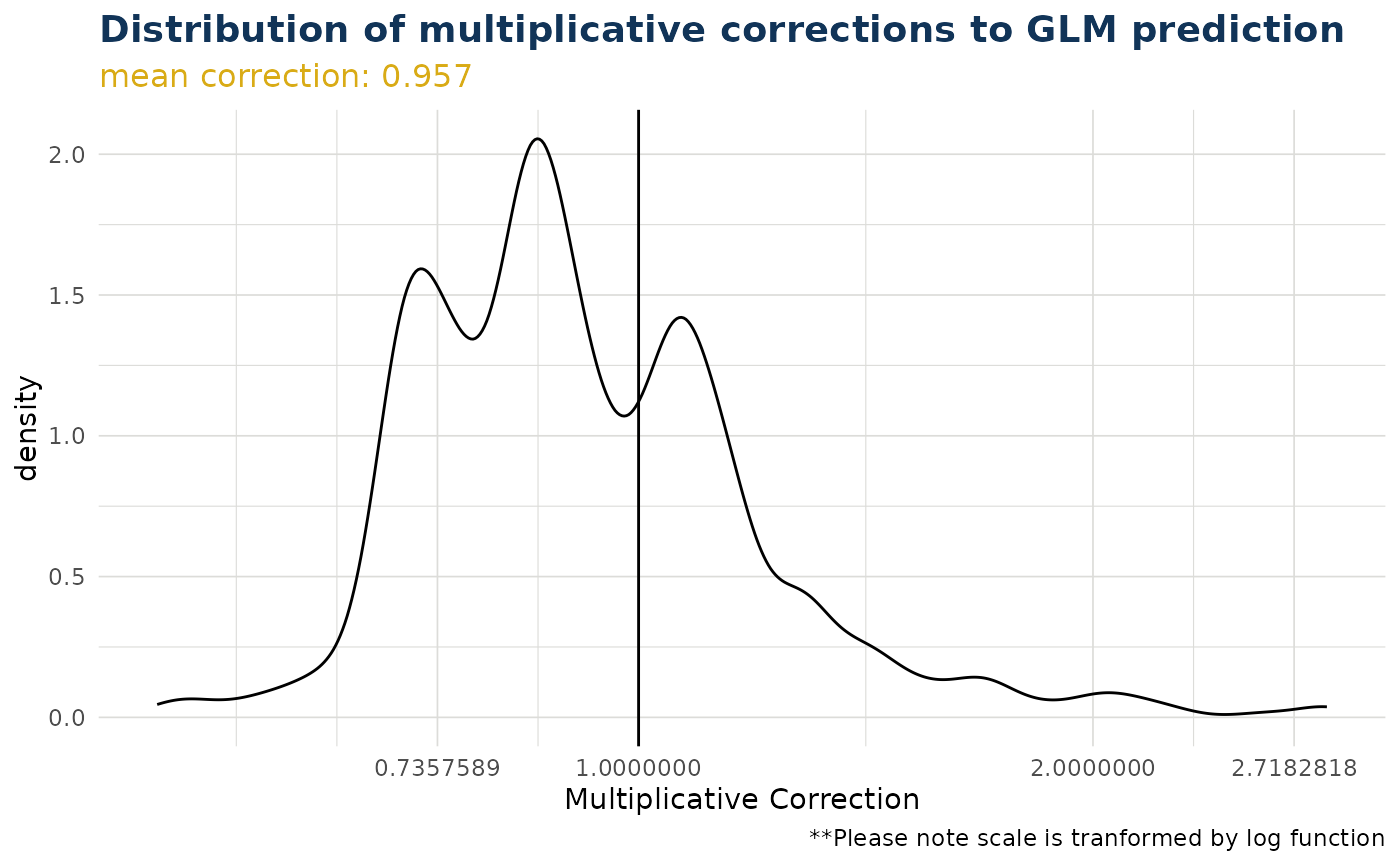
bias_density)- overall_correction
Function to show global correction distributions (see
overall_correction)- shap
Dataframe showing raw SHAP values of data records
- beta_corrections
Dataframe showing beta corrections (in wide/one-hot format) of data records
- data_beta_coeff
Dataframe showing beta coefficients of data records
Details
The following outputs are functions that can be called to create plots:
beta_corrected_scatter
beta_corrected_density
bias_density
overall_correction
For each of these, the key data arguments (e.g. data, shap, iblm_model) are already populated by `explain_iblm()`. When calling these functions output from `explain_iblm()` only key settings like variable names, colours...etc need populating.
Examples
df_list <- freMTPLmini |>
dplyr::mutate(LogExposure = log(Exposure), .keep = "unused") |>
split_into_train_validate_test(seed = 9000)
iblm_model <- train_iblm_xgb(
df_list,
response_var = "ClaimNb",
offset_var = "LogExposure",
family = "poisson"
)
ex <- explain_iblm(iblm_model, df_list$test)
# the output contains functions that can be called to visualise iblm
ex$beta_corrected_scatter("DrivAge")
#> `geom_smooth()` using method = 'gam' and formula = 'y ~ s(x, bs = "cs")'
 ex$beta_corrected_density("DrivAge")
 ex$overall_correction()
 ex$bias_density()
#> $bias_correction_var
ex$bias_density()
#> $bias_correction_var
 #>
#> $bias_correction_total
#>
#> $bias_correction_total
 #>
# the output contains also dataframes
ex$shap |> dplyr::glimpse()
#> Rows: 3,764
#> Columns: 7
#> $ Area <dbl> -4.487922e-03, 1.437818e-01, 1.612203e-02, -2.331074e-03, 1…
#> $ BonusMalus <dbl> -0.009690866, 0.072579175, -0.042828754, -0.063746683, 0.03…
#> $ DrivAge <dbl> -0.227601975, 0.191458955, 0.113016523, 0.114070870, 0.1605…
#> $ VehAge <dbl> 0.11503229, -0.27023473, 0.05617751, 0.11912487, 0.02605914…
#> $ VehBrand <dbl> -0.071816981, -0.153895795, 0.011852440, -0.030659221, -0.0…
#> $ VehPower <dbl> -0.016770046, -0.041518744, 0.018848389, 0.013932319, 0.024…
#> $ BIAS <dbl> -0.0301019, -0.0301019, -0.0301019, -0.0301019, -0.0301019,…
ex$beta_corrections |> dplyr::glimpse()
#> Rows: 3,764
#> Columns: 17
#> $ bias <dbl> -0.03010190, -0.03010190, -0.03010190, -0.03010190, -0.030…
#> $ BonusMalus <dbl> -1.425127e-04, 9.072397e-04, -8.565751e-04, -1.274934e-03,…
#> $ DrivAge <dbl> -7.341999e-03, 3.301016e-03, 2.897860e-03, 3.001865e-03, 3…
#> $ VehAge <dbl> 0.011503229, -0.270234734, 0.014044377, 0.009927072, 0.006…
#> $ VehPower <dbl> -0.0023957209, -0.0059312492, 0.0037696779, 0.0034830798, …
#> $ AreaA <dbl> 0, 0, 0, 0, 0, 0, 0, 0, 0, 0, 0, 0, 0, 0, 0, 0, 0, 0, 0, 0…
#> $ AreaB <dbl> 0.00000000, 0.00000000, 0.00000000, 0.00000000, 0.00000000…
#> $ AreaC <dbl> 0.000000000, 0.143781751, 0.000000000, 0.000000000, 0.0000…
#> $ AreaD <dbl> -0.0044879219, 0.0000000000, 0.0000000000, -0.0023310741, …
#> $ AreaE <dbl> 0.000000e+00, 0.000000e+00, 1.612203e-02, 0.000000e+00, 1.…
#> $ VehBrandB1 <dbl> 0, 0, 0, 0, 0, 0, 0, 0, 0, 0, 0, 0, 0, 0, 0, 0, 0, 0, 0, 0…
#> $ VehBrandB12 <dbl> 0.000000000, -0.153895795, 0.000000000, 0.000000000, -0.02…
#> $ VehBrandB2 <dbl> 0.00000000, 0.00000000, 0.01185244, -0.03065922, 0.0000000…
#> $ VehBrandB3 <dbl> 0.00000000, 0.00000000, 0.00000000, 0.00000000, 0.00000000…
#> $ VehBrandB4 <dbl> -0.07181698, 0.00000000, 0.00000000, 0.00000000, 0.0000000…
#> $ VehBrandB5 <dbl> 0.00000000, 0.00000000, 0.00000000, 0.00000000, 0.00000000…
#> $ VehBrandB6 <dbl> 0.0000000, 0.0000000, 0.0000000, 0.0000000, 0.0000000, 0.0…
ex$data_beta_coeff |> dplyr::glimpse()
#> Rows: 3,764
#> Columns: 7
#> $ bias <dbl> -3.841129, -3.841129, -3.841129, -3.841129, -3.841129, -3.8…
#> $ Area <dbl> -0.18551433, -0.06760171, 0.07351169, -0.18335748, 0.057532…
#> $ BonusMalus <dbl> 0.01828861, 0.01933836, 0.01757455, 0.01715619, 0.01889540,…
#> $ DrivAge <dbl> -0.0014584419, 0.0091845737, 0.0087814168, 0.0088854223, 0.…
#> $ VehAge <dbl> -0.01988902, -0.30162699, -0.01734788, -0.02146518, -0.0248…
#> $ VehBrand <dbl> -0.353582129, -0.049864996, -0.030394794, -0.072906455, 0.0…
#> $ VehPower <dbl> 0.05772452, 0.05418899, 0.06388992, 0.06360332, 0.06509935,…
#>
# the output contains also dataframes
ex$shap |> dplyr::glimpse()
#> Rows: 3,764
#> Columns: 7
#> $ Area <dbl> -4.487922e-03, 1.437818e-01, 1.612203e-02, -2.331074e-03, 1…
#> $ BonusMalus <dbl> -0.009690866, 0.072579175, -0.042828754, -0.063746683, 0.03…
#> $ DrivAge <dbl> -0.227601975, 0.191458955, 0.113016523, 0.114070870, 0.1605…
#> $ VehAge <dbl> 0.11503229, -0.27023473, 0.05617751, 0.11912487, 0.02605914…
#> $ VehBrand <dbl> -0.071816981, -0.153895795, 0.011852440, -0.030659221, -0.0…
#> $ VehPower <dbl> -0.016770046, -0.041518744, 0.018848389, 0.013932319, 0.024…
#> $ BIAS <dbl> -0.0301019, -0.0301019, -0.0301019, -0.0301019, -0.0301019,…
ex$beta_corrections |> dplyr::glimpse()
#> Rows: 3,764
#> Columns: 17
#> $ bias <dbl> -0.03010190, -0.03010190, -0.03010190, -0.03010190, -0.030…
#> $ BonusMalus <dbl> -1.425127e-04, 9.072397e-04, -8.565751e-04, -1.274934e-03,…
#> $ DrivAge <dbl> -7.341999e-03, 3.301016e-03, 2.897860e-03, 3.001865e-03, 3…
#> $ VehAge <dbl> 0.011503229, -0.270234734, 0.014044377, 0.009927072, 0.006…
#> $ VehPower <dbl> -0.0023957209, -0.0059312492, 0.0037696779, 0.0034830798, …
#> $ AreaA <dbl> 0, 0, 0, 0, 0, 0, 0, 0, 0, 0, 0, 0, 0, 0, 0, 0, 0, 0, 0, 0…
#> $ AreaB <dbl> 0.00000000, 0.00000000, 0.00000000, 0.00000000, 0.00000000…
#> $ AreaC <dbl> 0.000000000, 0.143781751, 0.000000000, 0.000000000, 0.0000…
#> $ AreaD <dbl> -0.0044879219, 0.0000000000, 0.0000000000, -0.0023310741, …
#> $ AreaE <dbl> 0.000000e+00, 0.000000e+00, 1.612203e-02, 0.000000e+00, 1.…
#> $ VehBrandB1 <dbl> 0, 0, 0, 0, 0, 0, 0, 0, 0, 0, 0, 0, 0, 0, 0, 0, 0, 0, 0, 0…
#> $ VehBrandB12 <dbl> 0.000000000, -0.153895795, 0.000000000, 0.000000000, -0.02…
#> $ VehBrandB2 <dbl> 0.00000000, 0.00000000, 0.01185244, -0.03065922, 0.0000000…
#> $ VehBrandB3 <dbl> 0.00000000, 0.00000000, 0.00000000, 0.00000000, 0.00000000…
#> $ VehBrandB4 <dbl> -0.07181698, 0.00000000, 0.00000000, 0.00000000, 0.0000000…
#> $ VehBrandB5 <dbl> 0.00000000, 0.00000000, 0.00000000, 0.00000000, 0.00000000…
#> $ VehBrandB6 <dbl> 0.0000000, 0.0000000, 0.0000000, 0.0000000, 0.0000000, 0.0…
ex$data_beta_coeff |> dplyr::glimpse()
#> Rows: 3,764
#> Columns: 7
#> $ bias <dbl> -3.841129, -3.841129, -3.841129, -3.841129, -3.841129, -3.8…
#> $ Area <dbl> -0.18551433, -0.06760171, 0.07351169, -0.18335748, 0.057532…
#> $ BonusMalus <dbl> 0.01828861, 0.01933836, 0.01757455, 0.01715619, 0.01889540,…
#> $ DrivAge <dbl> -0.0014584419, 0.0091845737, 0.0087814168, 0.0088854223, 0.…
#> $ VehAge <dbl> -0.01988902, -0.30162699, -0.01734788, -0.02146518, -0.0248…
#> $ VehBrand <dbl> -0.353582129, -0.049864996, -0.030394794, -0.072906455, 0.0…
#> $ VehPower <dbl> 0.05772452, 0.05418899, 0.06388992, 0.06360332, 0.06509935,…